Return-from-orbit Spaceplane Configurations with Varying Geometry, Missions, and Planetary Environments · Chapter 4

4.1Code Architecture

4.1.1User Settings

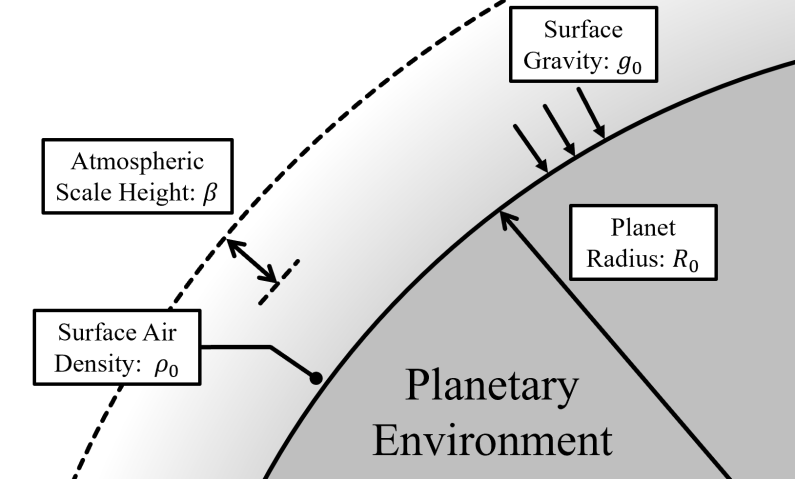
Assessing the performance of a spaceplane begins in the context of a planetary environment. The four parameters of a planetary environment (shown in Figure 4.1) are the first parameters loaded from a premade database of selected planets from reference [23] and a small set of hypothetical planets used to test the algorithm.

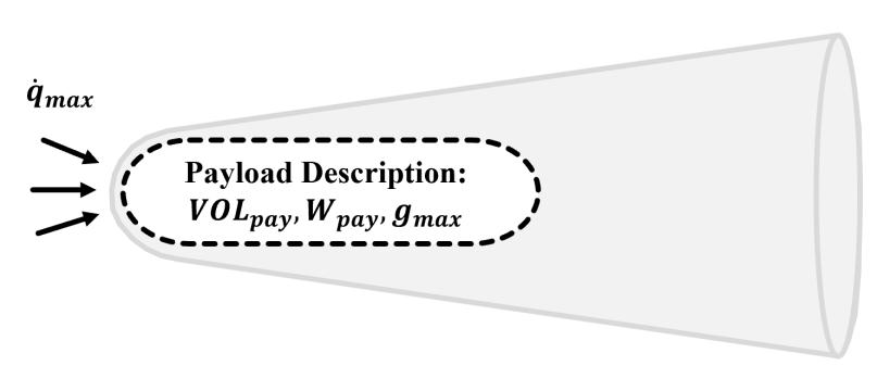
After a planet has been selected, the user adds a mission upon which the target spaceplane will be assessed. The mission is described by the weight and volume of the payload, the max g-loading to be endured by the payload, and the maximum heating rate to be endured by the craft. The last mission parameter is to be determined by the thermal protection system, but an estimate can be made based on current materials available.

As discussed in the previous chapter, the performance weight settings are also tweaked so that each of the normalized performance components can be fairly compared and considered by the algorithm. In practice, the payload fraction must be weighted so that the payload mass-weight is comparable to the structural mass-weight. In this way, parameters which measure inclination change are on the same order of magnitude. Of course, this is dependent on user preferences as each program has a different budget and goals.

For optimization, the user will set a few learning parameters which will be discussed in a later section. Without optimization, these are all set to a default of one.

4.1.2Assessment

Whether or not the configuration will be optimized, the algorithm takes a first guess or an existing configuration to assess. This is given in the order of the six geometric parameters presented at the beginning of the previous chapter. The five latter geometric parameters are input as being normalized the first (aft radius). In this way, during optimization, most of the parameters are not adjusted by their individual dimensions, but rather by their relation to the scale of the aft radius.

The performance is then assessed according to the mission and user-specified weights in the given planetary environment. The methodology for performance assessment is described in the previous chapter and encapsulated in a function.

During this assessment, a logic decides on the existence of a propulsion system depending on volume constraints. It also checks to see if the mission is viable. If not, performance values of zero will be output to let the algorithm know that the design is worthless in terms of meeting mission goals.

4.1.3Full Process

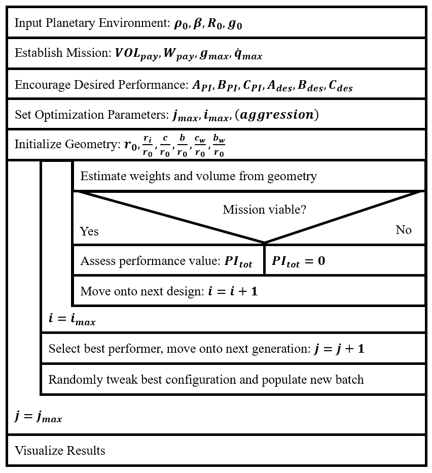
The code architecture is documented in the Nassi-Schneiderman Diagram shown in Figure 4.3. The loops are ignored at the default optimization settings (where $i=j=1$), so the main analysis for a point study can be summarized by the innermost loop process preceded by the initialization process.

4.2Results and Comparisons

4.2.1Trends in Geometry

The trends found in the geometric analysis are first analyzed. In keeping with trends for high-performing vehicles, the nose and aft radii are held fixed at $r_1=0.01r_0$. The wetted area can now by computed for varying values of chord and span, as shown in Figure 4.1.

After setting bounds to the chord and span adjustment, the results for changing wetted area are shown in Figure 4.5.

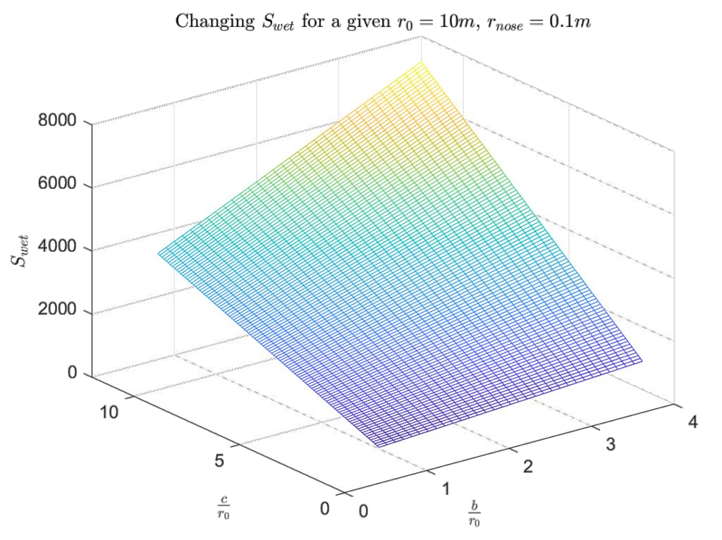
The wetted area is the primary determinant of the structural weight, which is to be used in performance calculations. This changing structural weight is plotted in Figure 4.6.

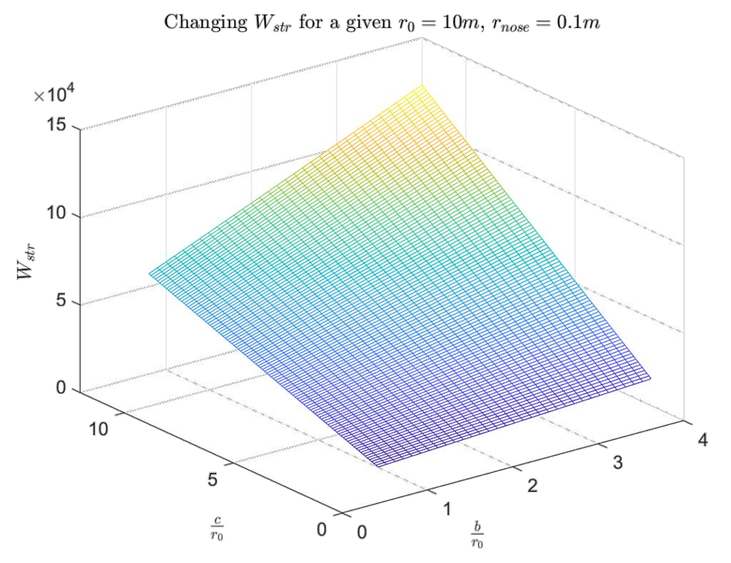
The wetted area is the primary determinant of the structural weight, which is to be used in performance calculations. At the same time, Küchemann’s Tau is competing with the structural weight. It is apparent by Figure 4.7 that the structural weight is inversely related to the tau parameter (take note that the x and y axes are inverted for the reader’s visibility).

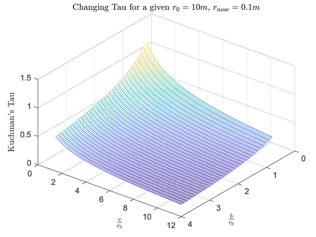
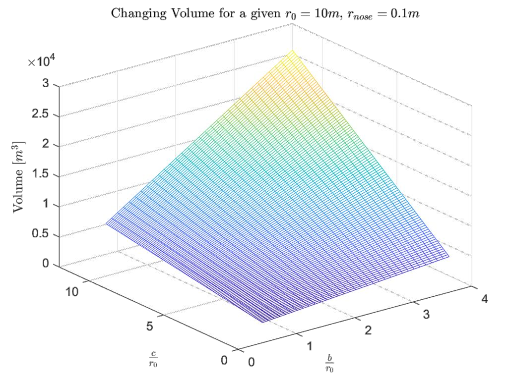
These two parameters must compromise with each other as the volume must remain fixed to meet the mission requirement and allow for a propulsion system with propellant if an inclination change is to be performed. The lowest Küchemann’s Tau yields the highest lift-to-drag ratio and highest aerodynamic performance. The total configuration volume available for payload, propulsion system, and propellant is plotted in Figure 4.8.

To see the full picture, the changing geometric results are now plotted for a changing nose radius. Of course, this is for a fixed chord and span so this plot can change along those dimensions, just as the 3-dimensional plots can changed along a third axis of nose radius size.

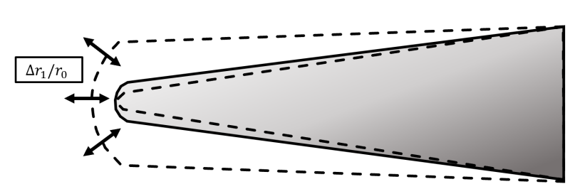
Since only one parameter is being adjusted, the geometric analysis can be conducted on one plot with different lines separated by output category.

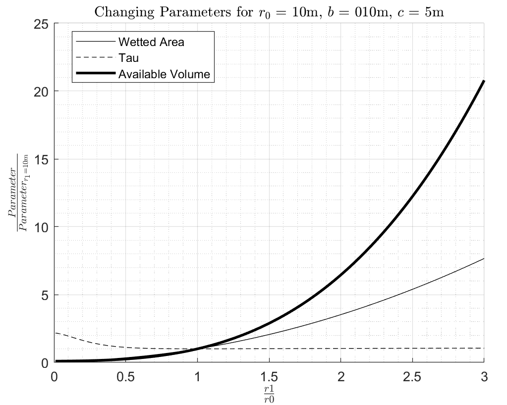
It is interesting to see that Küchemann’s Tau is remaining roughly constant after the nose radius is about half of the aft radius. This is because tau is a function of shape, and once the nose increases past a certain point, the shape becomes dominated by the nose radius. Since the values are normalized, the trends for wetted area and structural weight are equivalent.

The author has observed that one of the most frequently changing parameters during optimization other than aft-radius scaling was the chord length in relation to the aft radius. The vehicle parameters are now observed for a changing chord length. An increase in chord length increases the available volume for propellant, decreases tau, but rapidly increases structural weight. Figure 4.11 shows the basic geometry parameters changing as a function of chord.

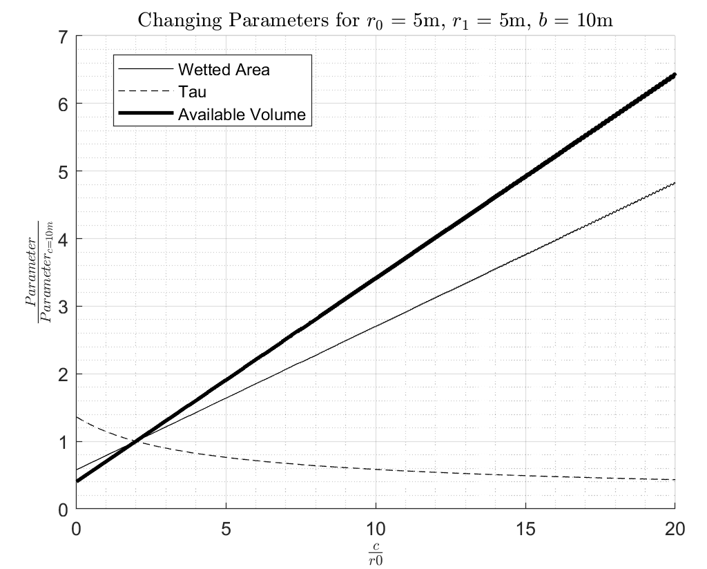
Tau appears to be more well-behaved than when it was changing with respect to an ellipsoid shape expanding (increasing nose radius), and the wetted area and volume are increasing linearly as expected for a simple extrusion. Due to the radii being equal, this is equivalent to the “pill” shape expanding. The author arbitrarily selected this as the nominal condition, but any other combination of variables deviating from the nominal pill will also demonstrate a linear relationship in the same way that volume and area scales linearly with height regardless of cross section (for instance, stretching a cone would change its parameters linearly). Even with stretching, the change in tau is non-linear as it is a power relationship between two scaled heights. Additionally, it is unreasonable for tau to become negative by its definition, so one would expect its value to decay as a function of shape.

The inclination change capability of the vehicle is now assessed with respect to increasing chord in Figure 4.12, which is assessed for the planet Jupiter.

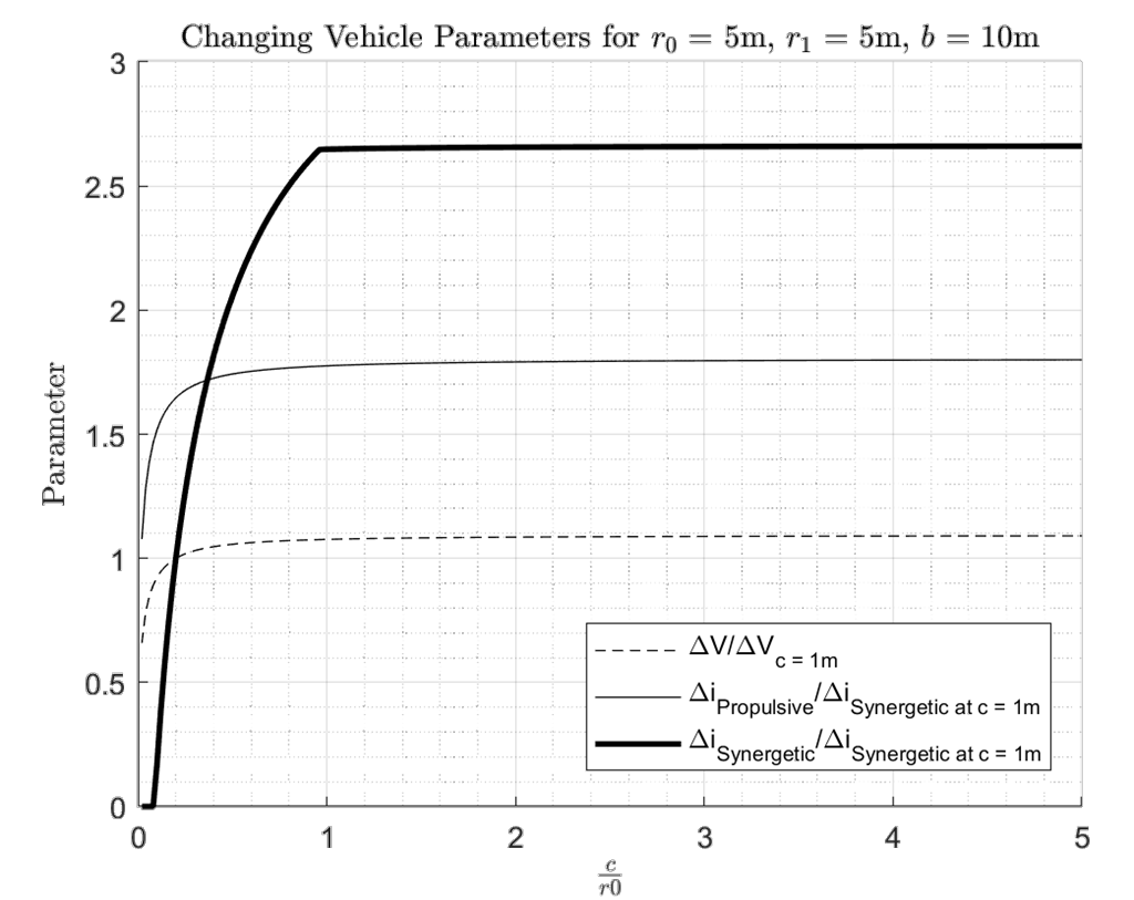
This is certainly a plot which proves the utility of a synergetic maneuver. Firstly, increasing chord length will increase $\mathrm{\Delta }{V}_{available}$, but only up to a point. At this point, the increase in structural weight outweighs the benefit gained from increased value from gaining volume for propellant. This is why staging in a rocket greatly reduces the launch weight, since in a staged rocket, the velocity increment slope with increasing size is more of a steep linear line than a shallow asymptotic curve.

Given the $\mathrm{\Delta }{V}_{available}$, an inclination change can be made in one of two ways: a synergetic maneuver (where aerodynamic capability comes into play) or a purely propulsive maneuver. It is shown that after a certain point with respect to the nominal value of a 1-meter chord, higher inclination change gains require employing the synergetic maneuver. Moreover, since the maximum $\mathrm{\Delta }{V}_{available}$ is finite (with different finite values according to configuration constants), the change in inclination has a finite maximum, and only the synergetic maneuver can achieve the complete turn from an equatorial to a polar orbit.

4.2.2Data Points

In this subsection some arbitrarily selected configurations will be assessed to build a database of initialization vectors for optimization.

The study will begin with assessing variations of the geometric trends with the categories of nose-to-aft ratios. It will then move on to superimposing wings, including an unrealistic low-sweep angle design which is not structurally feasible. However, this configuration will be useful for determining the bounds of the study.

• Big Nose
• Constant Nose
• Small Nose
• High Sweep Wing
• 45-degree sweep wing
• Low sweep wing

4.2.3Historical Designs

This subsection will assess the accuracy of the performance assessment with real-world analogues. Correction factors and future analysis work will be discussed in the context of the findings. These designs can also serve as starting points (or target points) for optimization.

• Model 176
• Dream Chaser
• Dyna Soar Multi-Planet performance
• Space Shuttle
• Apollo 11 Capsule

4.3Optimization

4.3.1Methodology

The methodology for optimization begins with an initialized geometry vector, which represents any arbitrary configuration. The hope of optimization is that even a low-performing starting configuration will evolve into something realistic or useful after a given number of iterations.

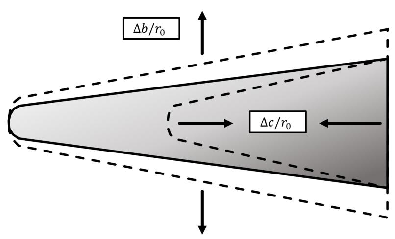
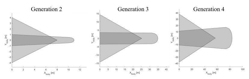
The methodology of the optimization routine is inspired by the theory of biological evolution, where a design will be subjected to an environmental requirement and selective pressures, and only the best-performing designs will be allowed to have offspring. Of course, for the design to improve on learned attributes, the offspring of the best-performing configuration will resemble the parent. However, according to the aggressiveness of the learning rate, some of the children will be mutated in different ways. From here, the best performing child is assessed and used to populate the next generation. This process is visualized in Figure 4.13.

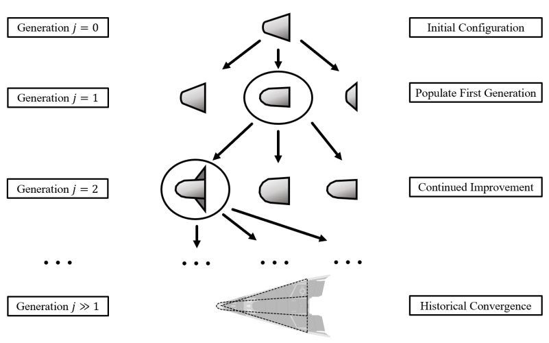
As can be observed in Figure 4.13, the mutation function includes a small chance to spawn a wing. Conversely, a wing can be randomly removed. If a wing is detrimental to performance, its structural cost will cause children without it to be more successful than their peers.

Relating the evolution analogy to the mathematical reality, the optimization routine here is akin to a traveler along a multi-dimensional topology looking for a local minimum. Local minimums are numerous for these many parameters, which is why the screening of initialization values is necessary to find the best local minimum. The “mutations” are akin to small steps in random directions all at once in this topology. An increased number of children per generation relates to more steps in random directions per step, giving the traveler a better picture of where next to step. The aggressiveness of the mutations determines the size of these steps. Larger steps may converge on a solution faster, but it will increase the chance of divergence.

If all except two of the geometric parameters were held constant, the topology could be visualized in a 3-dimensional plot useful for visualizing the concept of the optimization routine (the topology shown in Figure 4.14 is from reference [24] for illustrative purposes and is not numerically representative of the actual topology produced by the author).

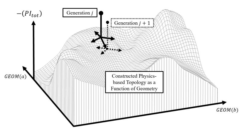
The number of steps taken per generation is analogous to the number of children per generation (this is the algorithm batch setting, with a default of $i=1$). The best “step” is taken to the next generation. The number of non-trivial steps will always be less than or equal to the batch size, as not every offspring will mutate for low levels of aggression.

4.3.2Results

The author initializes an early test of the algorithm with a non-sensical configuration employing a large nose and small wing. Evidently, the aerodynamics of such a craft are not efficient nor sized optimally for a mission with a payload of 100 kg and a volume of 10 m³. The following figures show the top-view of the evolving configurations.

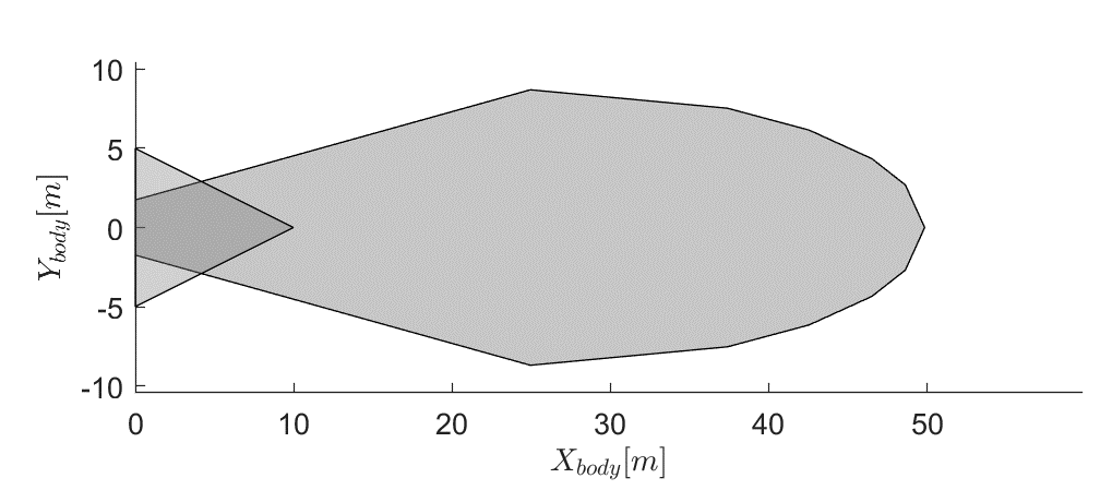
From here, the optimization routine takes small steps toward better-performing vehicles with each successive generation.

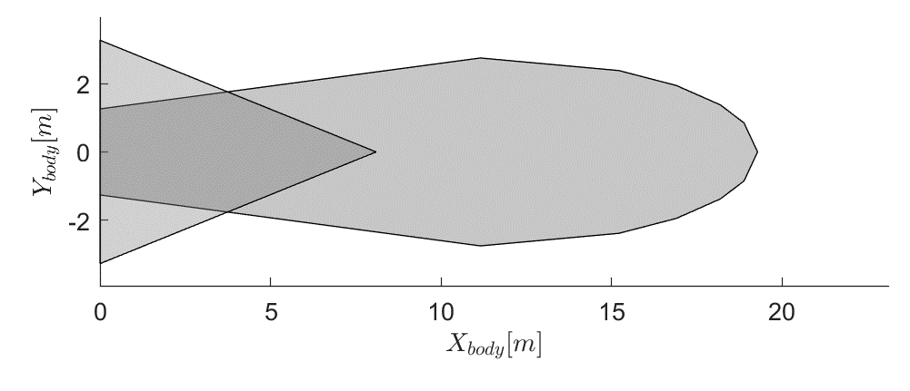
As shown by the axes of Figure 4.16, it is apparent that the most noticeably changed aspect of this configuration is the overall scale of the vehicle. This is due to the way the configuration’s geometry vector is set up. The values are all with respect to element GEOM(1), which is the aft radius. Any change to this value will directly scale the rest of the design with it. In this way, the mutation function has an avenue of scaling the entire craft at once.

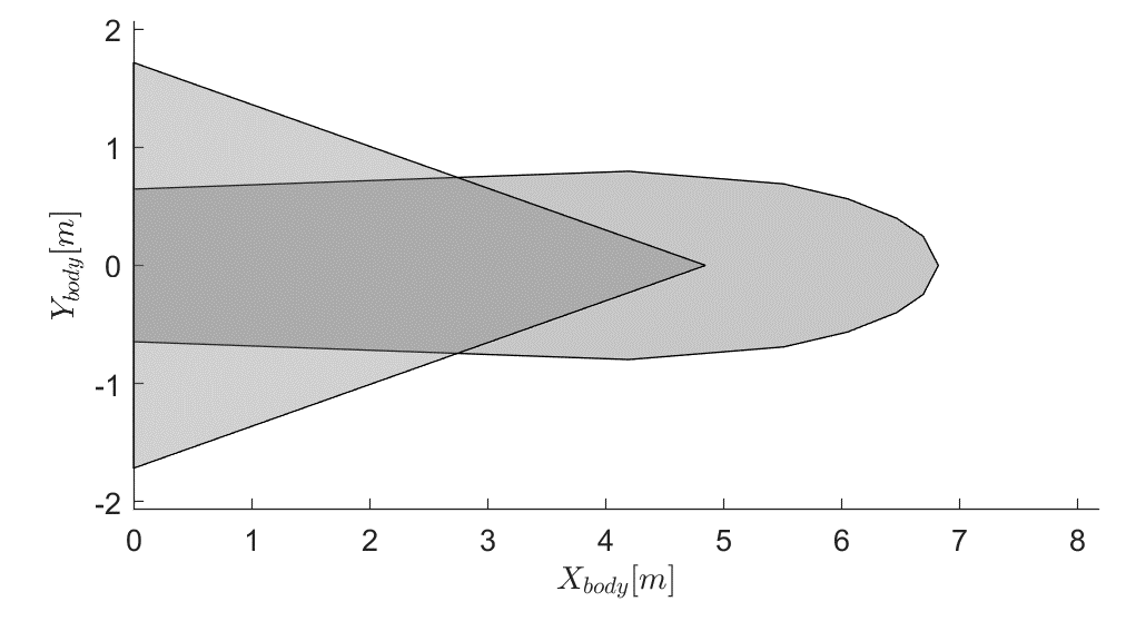
The configuration in Figure 4.17 is among the last with propulsive capability, as the weights were such that payload capability is increasingly favored over an inclination change. However, the $\mathrm{\Delta }{V}_{available}$ for this configuration is 2.40 km/s with an engine achieving 350 seconds of specific impulse. Based on the aerodynamic capability of the Figure 4.17 configuration, the craft can only perform a propulsive inclination change. This is likely attributed to an inaccurate lift-to-drag estimation from a high tau value (which is a result of the desire to increase the payload fraction).

The key to a successful convergence is to find the correct costing function weights to teach the algorithm what the user is looking for. The first successful convergence had a very high payload fraction logic-weight, and resulted in the configuration seen in Figure 4.18.

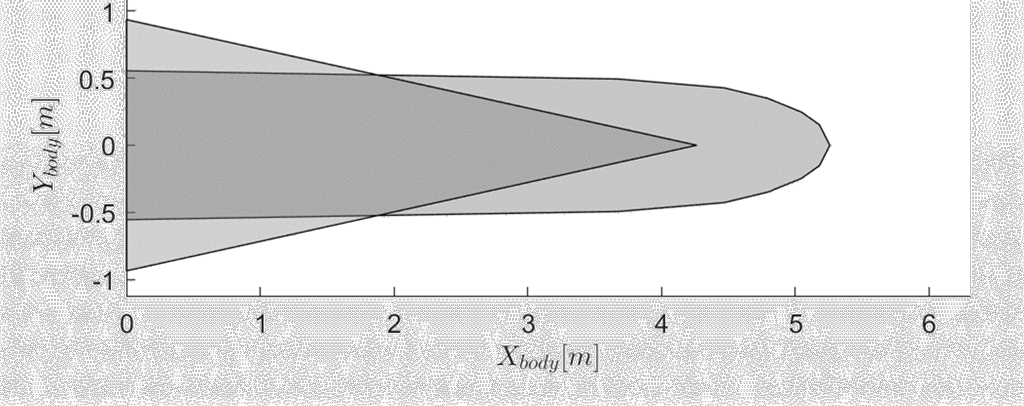
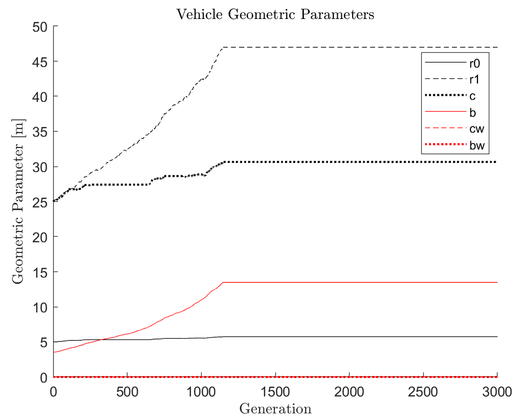
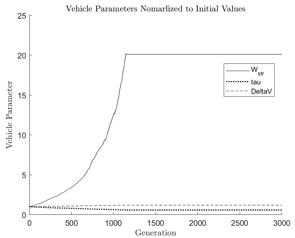
The conclusion of this first attempt was that there was too much emphasis placed on decreasing the structural weight. Such user-settings cause the algorithm to converge on a minimum-volume capsule design with residual wings. The geometric evolution and vehicle capabilities across these 3000 generations is plotted in Figures 4.19 and 4.20.

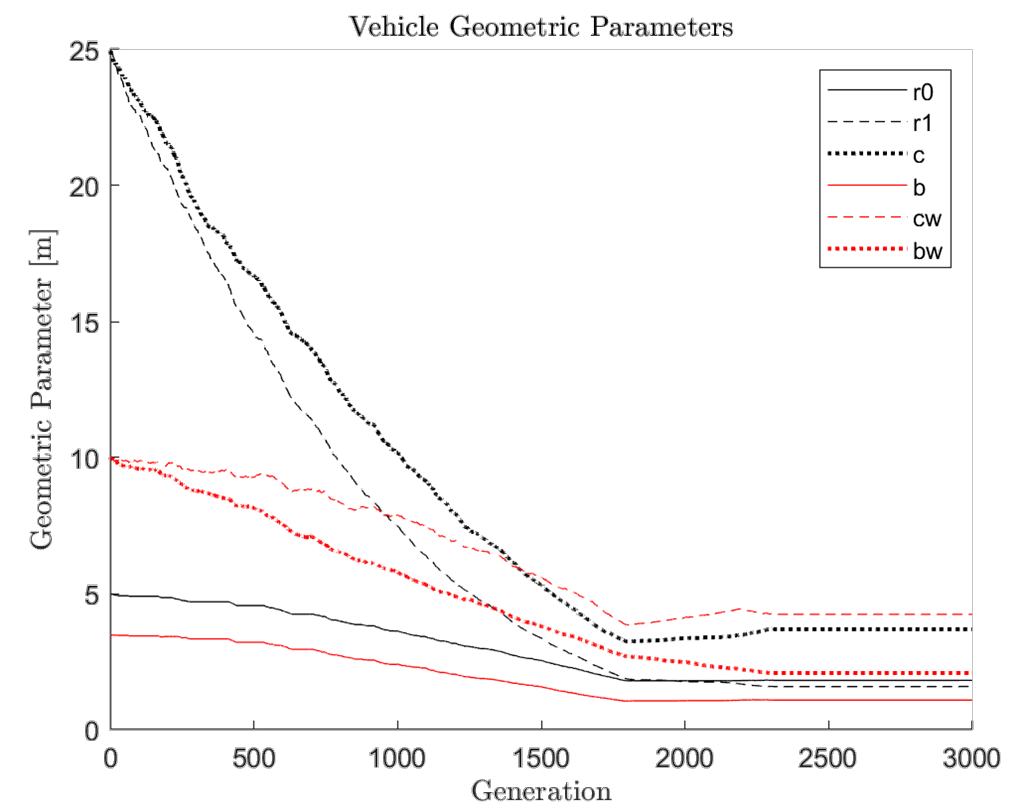
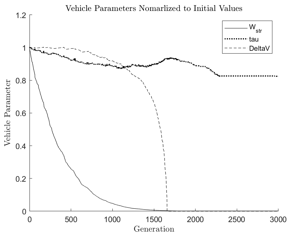
In earlier unsuccessful convergence trials, the logic-weight for inclination change performance was set to dominate the logic-weight for payload fraction. This happens when the weights are equal to each other, as the payload fraction performance index tends to be very small due to the relationship between payload density at required structural weight to encapsulate it. Additionally, the density of the of the propellant will further exacerbate the trade-off between propulsive capability and payload capability. For these reasons, without a mission failure trigger, the algorithm will ignore the payload capability and focus on increasing the aerodynamic and propulsive capabilities. Fortunately, the model for estimating lift-to-drag has been set up to cap the performance to $L/D=3$ according to conservative historical expectations [7]. As a result of this cap, the algorithm has little reason to continue slenderizing past the tau value associated with the $L/D$ cap. It is worth noting that there is a minimum bound as well, which is why the Figure 4.17 configuration was assumed to be ballistic (obviously by observation, this estimation model must be modified to include low-performing configurations). After iterating using these weights the configuration converges to the configuration seen in Figure 4.21.

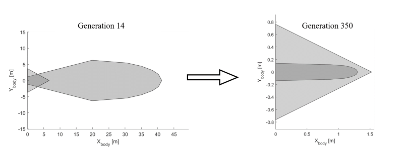
Using the alternative method of lift-to-drag estimation, the geometry converges to form a capsule shape.

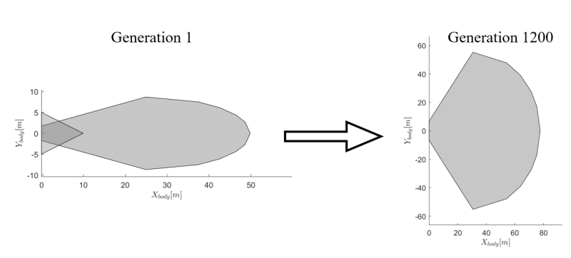
The geometric evolution of this lineage is shown in Figure 4.23. It converged in about half the time as the first convergence.

The vehicle parameters in Figure 4.24 show that the velocity change available is relatively constant. The tau value changes in the same way that it would with an increasing nose radius.

4.3.3Observations

The algorithm exploited an earlier convergence attempt when the author neglected to factor in the nose section into the structural weight. While it did increase the loft section’s wetted area, the growing nose area was not computed, so it became more advantageous to grow this section unrealistically.

Spotted an error, or want to reply? Email me: leonardo.pinero42 [at] gmail [dot] com