IILiterature Review

Author: Leonardo Pinero-Perez
Written: 2018 · Report, University of Texas at Arlington
Original: Full report · 120 pages
Contents: Nomenclature · Chapter I · II · III · IV · V · VI · VII · VIII · IX · X · XI · Appendix · References
Ref: MAE 4351-2018

Converted from the original PDF on 8 Nov 2026 with Claude Opus 5.5. The wording is unchanged, except: two classmates’ names are replaced by their roles, Figure 54 (an attendance sheet) is omitted, and my name is spelled without accents. Equations, figures and numbering follow the original. Conversion not yet checked against the PDF.

AManagement

As the lead chief engineer, the author has realized that there is in fact a learning curve to developing the skills necessary to extract maximum productivity from the team. This section will provide some sources for managing the team which led to the project deliverables. This section is relevant to an engineering report since the process for managing directly influences the effectiveness of the engineering methodology described.

There are many books on leadership and business development, so it is important to select relevant sources. References were selected by the ethos of the writers of these books. Writers were selected by their individual accomplishments in the technology industry, since this industry is based on a product which must be engineered (thus relevant to this engineering project).

The writers selected are listed below:

Peter Theil, founder of PayPal and Palantir Analytics [7]
Ben Horowitz, CEO/founder of Opsware [8]
Andrew Grove, cofounder and CEO of Intel [9]

Peter Theil’s book Zero to One is useful as a primer to the idea of startups and their place in American and global culture. Being a short book, it does not give highly specific methods of management, but many of the chapters are good for insights on the place of our project as an engineering deliverable to the rest of the world and its goals.

Ben Horowitz’s book Hard Things has been very useful on the details of managing a large company and developing methods of communication and business-side strategy. It is lacking in engineering expertise and product development, although the book seems to have been meant for engineers-turned-managers. Even so, the human element in the author’s role is significant, so this book is still relevant. Some useful principles drawn from this book:

When hiring a management team, most startups focus exclusively on IQ, but a bunch of high-IQ people with the wrong kind of ambition won’t work.

Perhaps the CEO’s most important operational responsibility is designing and implementing the communication architecture for her company.

This communication architecture might include [8]:

Organizational Design
Meetings
Processes
Email/Yammer
One-on-one meetings

The source has an entire chapter dedicated to setting up one-on-one meetings with employees to extract as much productivity and direction from the organization as a whole. One-on-one meetings are also referenced in Dr. Grove’s book High Output Management, which is actually referenced in Horowitz’s book.

Not much information has yet been extracted from Andrew Grove’s High Output Management since this book has not been read completely by the time of this report’s writing. However, the book’s introduction does explain what type of information the reader can gain from reading it. The performance measures of a manager are stated, and the book explains how a manager can increase that performance measure from a manufacturing point of view (every working organization has a product, such as the intellectual property of an engineering group).

The output of a manager is the output of the organizational units under his or her supervision or influence. [9]

In his book, Dr. Grove explains the concept managerial leverage, which measures the influence a manager has on the productivity of his or her team. The productivity of a manager is determined by the way managerial leverage is exercised. The book goes over how to exercise such leverage effectively and as much as possible. This has to do with task-relevant feedback [9].

BCost

A useful resource for numerically determining costs of a program or individual vehicle after the first iteration is the NASA Cost estimating handbook [10] and the older NASA Spacecraft Cost Estimation report [11]. The cost will be calculated when the first iteration is completed, so that future iterations can be optimized for commercial missions. The methodology from this handbook is outlined in the Nassi-Schneiderman diagram below.

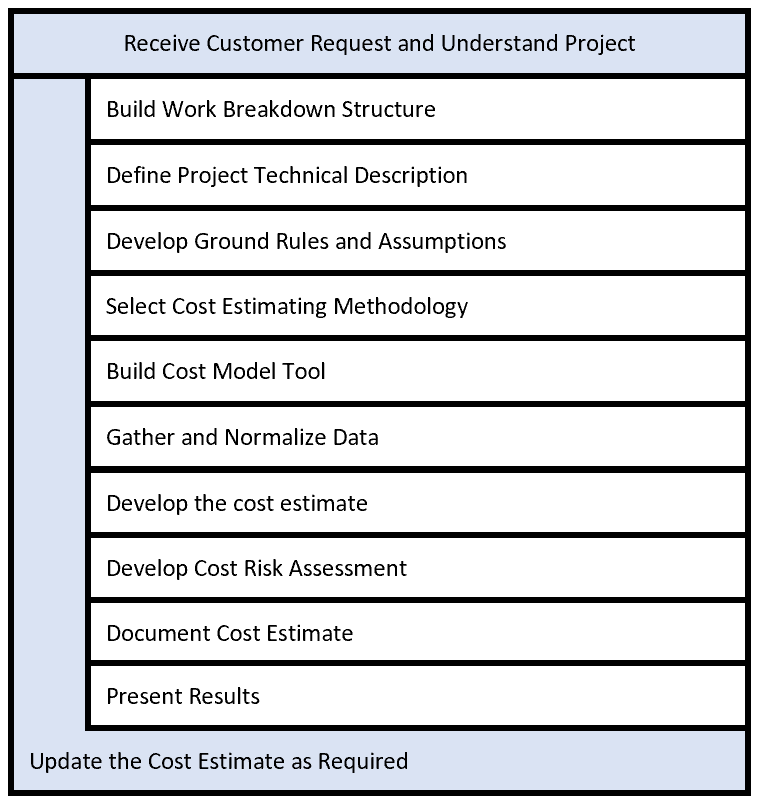
Nassi-Schneiderman diagram of the cost-estimating process: receive the customer request and understand the project, build the work breakdown structure, define the technical description, develop ground rules and assumptions, select the methodology, build the cost model, gather and normalize data, develop the estimate and its risk assessment, document and present the results, and update the estimate as required. — Figure 6Nassi-Schneiderman Diagram for the NASA Cost Estimating Handbook

The first step requires an understanding of the project, and from here a work breakdown structure can be built.

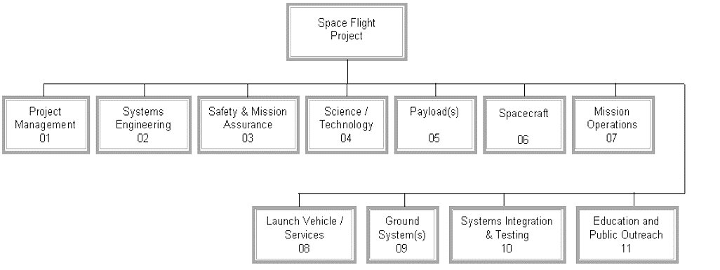
Text panel of four groups of questions to ask before a cost analysis, headed Data, Expectations, Resources and Schedule. — Figure 7Four Critical Elements Related to Conducting and Understanding a Cost Analysis *[10]*

Below is an example work break down structure (WBS) and will be used as inspiration for developing Ascension Aerospace’s completed and anticipated activities.

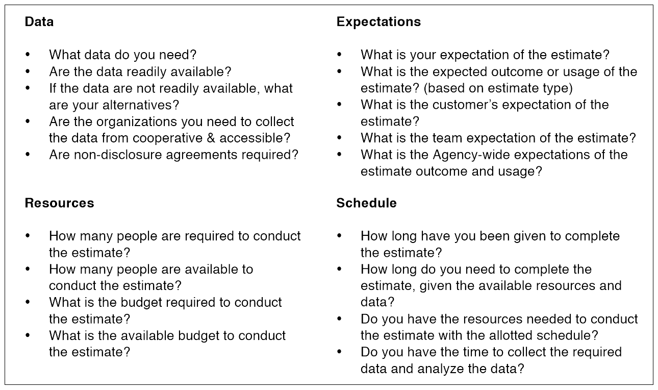
Organization chart of a space flight project’s level 2 work breakdown structure, with eleven elements numbered 01 to 11: project management, systems engineering, safety and mission assurance, science and technology, payloads, spacecraft, mission operations, launch vehicle and services, ground systems, systems integration and testing, and education and public outreach. — Figure 8Standard NASA Project Level 2 Work Breakdown Structure *[10]*

After a WBS is made, the project must be defined and estimation ground rules established. Defining ground rules and assumptions may include the following [10]:

Scope: this is largely defined by the WBS
Make vs. buy decisions: do you develop an engine or buy off-the-shelf?
Government Furnished Equipment/Information (GFE/GFI): the government (or other organizations) may provide technical capabilities and assistance or information which could drive down program costs. This assumption allows the free development of technology and products which fall under this category
Contractors and Subcontractors: similar to buying off-the-shelf, but for research and development
Budget profile: predicts the effect that a budget will have on the overall cost
Labor resources and rates: this is dependent on program location and availability of labor for specific skill sets
Risks and associated risks: if risk mitigation measures are put into place, they will increase the baseline cost estimate but reduce cost overruns
Production units and quantities: increased quantities, as with flight frequency described later in this section, can drive down costs per unit
Description of dollars and inflation: this is especially useful for programs that run for several years

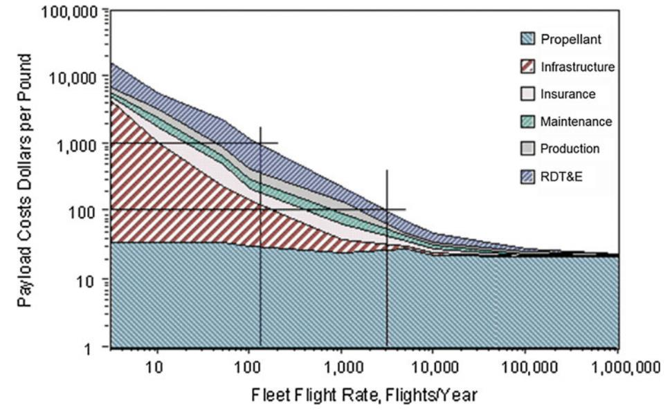
A useful plot was found suggesting that operational costs drastically reduce with increasing flight frequency. This is because existing infrastructure can be used multiple times to support increased flight frequency, driving down the cost of LEO transport. [2] The image below will be referenced as a guide for reducing cost. Keeping in mind that the plot is logarithmic, the biggest cost drivers are research and development, reusability, and infrastructure. The latter two can be greatly reduced by designing a reusable craft with rapid turn-around time [2].

Stacked area chart on log scales of payload cost in dollars per pound against fleet flight rate in flights per year, from 10 to 1,000,000, split into propellant, infrastructure, insurance, maintenance, production and RDT&E; the total cost falls steeply as the flight rate rises. — Figure 9Payload Cost per Pound vs. Flights per Year *[2]*

CSynthesis

The sizing method currently under consideration is the Czysz method [2], which takes the industry capacity index (ICI) into account to determine which geometries are possible for a given planform and structural ratios. The required ICI is what represents mission requirements such as payload volume and delta V. These mission requirements size the aircraft for a given payload size. Ideally, the most cost-effective design with the lowest ICI in the solution space which can carry the required payload. One such space found in [2] is demonstrated:

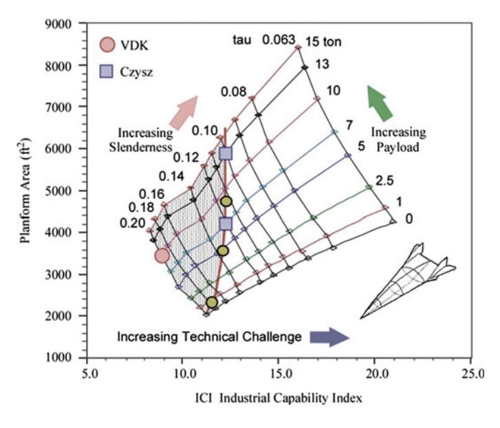
Carpet plot of planform area in square feet against the industrial capability index, with lines of constant tau (0.063 to 0.20) and constant weight (1 to 15 tons); data points from VDK and Czysz, and arrows marking increasing slenderness, increasing payload and increasing technical challenge. — Figure 10Czysz Sizing Method found in Literature *[2]*

The sizing process begins with defining certain based on disciplinary available technology and mission requirements. The coefficients are defined as follows:

I C I = 10 * \frac{I_{p}}{I_{s t r}} = 10 * \frac{(\frac{ρ_{p p l}}{W_{R} - 1})}{(W_{s t r} / S_{w e t})}

I_{p}

is a function of propulsive technology and delta V required, and

I_{s t r}

is dependent on advancement in material and structural design. Together, they formulate the industrial capacity index. The

I_{p}

is further described by [2]:

I_{p} = [\frac{ρ_{f u e l} (1 + r_{O / F})}{1 + r_{O / F} * \frac{ρ_{f u e l}}{ρ_{o x i d i z e r}}}] {\exp [\frac{Δ V * \frac{T}{D}}{g * I_{s p} * (\frac{T}{D} - 1 - \frac{\sin γ}{(\frac{T}{D})}}] - 1}^{- 1}

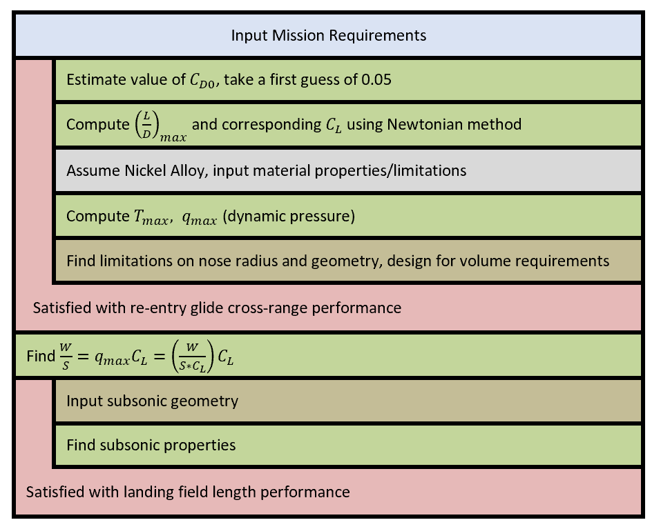
It is planned to use Corning’s method as inspiration for the development of a methodology to select key design variables early on and will be used as a testing ground for the methodologies of each of the disciplines when they are asked to provide deliverables. In this book, chapter two outlines this early methodology for the design of re-entry vehicles [12]. The Nassi-Schneiderman diagram of this method has been built to use as a comparison to the methods developed by the author. The process found in Corning’s book provided inspiration for the important variables in disciplinary analysis.

Nassi-Schneiderman diagram of Corning’s method: input mission requirements; estimate the zero-lift drag coefficient, compute the maximum L/D and its lift coefficient, assume a nickel alloy, compute the maximum temperature and dynamic pressure, and find limits on nose radius and geometry until the re-entry glide cross-range is satisfied; then find the wing loading and subsonic geometry and properties until the landing field length is satisfied. — Figure 11Nassi-Schneiderman Diagram for Corning's Method for Re-entry Vehicle Characteristics

DPerformance

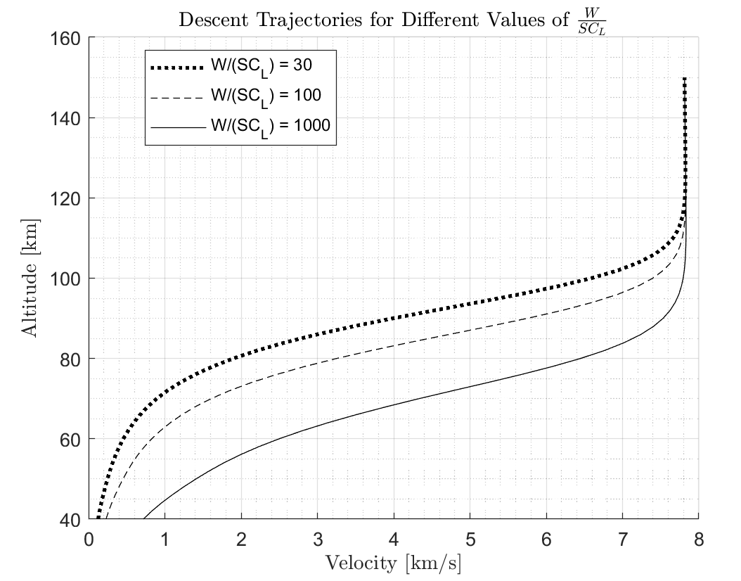
A good source for performance and re-entry trajectories was Gerald Corning’s book on Aerospace Vehicle Design [12]. This was an inspiration on where the author could start developing a trajectory-based MDA. The following plots are what drive the design based on mission requirements for cross-range capability. The following plot describes the descent trajectory for a vehicle of given aerodynamic characteristics following a line of constant dynamic pressure (that is what these characteristics solve for). This constant dynamic pressure determined by the lifting characteristics of the body implies that this is a steady state descent, but this plot is not useful to determine the rate of speed decay due to drag. To determine this, the ballistic coefficient must be known, which is based on drag characteristics and a different area of the vehicle. The equation which describes the trajectory according to the key design parameter is written below.

V_{v e h i c l e} = {[\frac{1}{V_{C}^{2}} + \frac{ρ}{2 (\frac{W}{S C_{L}})}]}^{- \frac{1}{2}}

The variable $V_{C}$ defines the circular velocity speed, which is the velocity required to maintain a circular orbit at that altitude. This is a function of altitude in a similar way as the function for atmospheric density. It is interesting to note that all of the velocity keeping the vehicle in the air is due to $V_{C}$ in orbit, where the density is equal to zero. The equation will show this truth with this extreme case: the forces keeping the vehicle afloat are a combination of aerodynamic lift and orbital velocity.

The author plotted this equation in MATLAB, trying to visualize different values for different hypothetical descending craft. Their descents are shown below and the script is found in the appendix.

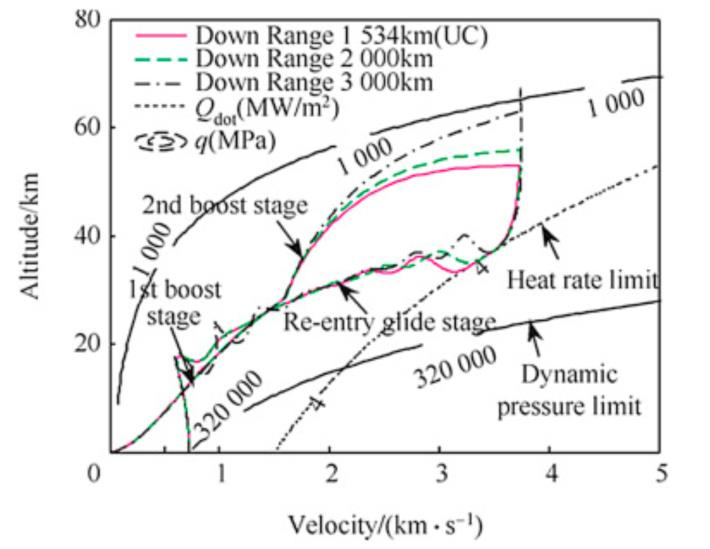
Plot titled “Descent Trajectories for Different Values of W/SC_L”: altitude in km against velocity in km/s, one glide curve each for W/(SC_L) = 30, 100 and 1000; all descend from about 150 km at about 7.8 km/s, the lowest value gliding highest. — Figure 12Descent Trajectory based on Changing Design Parameters

The following trajectory plot can be used to bleed speed or prove that it is easy to escape the atmosphere solely by aerodynamic maneuvering. As was described in the historical background, this has a precedent in the Silber Vogel design and allows for increased range by skirting through several sub-orbital paths. This was theorized in the Amerika Bomber in German designs to increase the range of military aircraft before and during World War II [13].

Chart of altitude in km against velocity in km/s for three down ranges of 1,534 km, 2,000 km and 3,000 km, showing the first and second boost stages and the re-entry glide stage between lines of heat-rate limit and dynamic-pressure limit. — Figure 13Dynamic Soaring Trajectory Plot *[14]*

A summary of the lit review found by the Performance discipline is described below [15]:

Convective heating for vehicle geometry and velocity:

{\dot{q}}_{c o n v} = 15 {(\frac{ρ_{\infty}}{R_{0}})}^{0.5} {(\frac{V_{\infty}}{1000})}^{3} (\cos Δ)^{1.5}

Stefan-Boltzmann’s equation (for outgoing radiation heating rate):

θ_{w} = {[\frac{{\dot{q}}_{c o n v}}{ε υ_{S B}}]}^{\frac{1}{4}}

EAerodynamics

The aerodynamics database can be found in Section A of the Appendix and a more detailed literature search in their respective reports. A summary of this discipline’s literature research is shown below [16]:

Useful References:

Anderson, J. D., Hypersonic and high-temperature gas dynamics, Reston: AIAA, 2006.
Anderson, John D., Jr., “A Survey of Modern Research in Hypersonic Aerodynamics,” AIAA Paper 84-1578, June 1984.
Anderson, John D., Jr., “Hypersonic Viscous Flow over Cones at Nominal Mach 11 in Air,” ARL Rept. 62-387, Wright-Patterson Air Force Base, OH, July 1962.
Draper, A. C., and Sieron, T. R., “Evolution and Development of Hypersonic Configurations 1958-1990”, Final Report for Period July 1990 to March 1991, Flight Dynamics Directorate, Wright Laboratory, Air Force Systems command, Wright-Patterson AFB, OH, Sep. 1991.
Dunbar, B., “NASA Dryden Fact Sheet - Lifting Bodies,” NASA Available: https://www.nasa.gov/centers/armstrong/news/FactSheets/FS-011-DFRC.html.
Nicolai, L. M., and Carichner, G. E., Fundamentals of Aircraft and Airship Design: Aircraft Design; Volume I, Reston, VA: AIAA, 2010.

The Anderson books are used to develop the methodology for hypersonic aerodynamic variables. Draper and Dunbar are historical references on hypersonic geometry development. Nicolai’s design book will be used to develop the subsonic-supersonic methodology for Wing & Airfoil Selection and Drag Build-up.

Estimation Equations [16]:

{(\frac{L}{D})}_{m a x} = \frac{A}{M} (M + B)

C_{D 0} = \frac{0.05772 . \exp (0.4076)}{β} = \frac{0.087}{\sqrt{M^{2} - 1}}

C_{D} = C_{D 0} (1 + B)

Parameters A and B are regression values to a trendline depending on what is considered state-of-the art. These values improve over time, ranging from 3 in the 1960’s to 4 in the foreseeable future [2].

FPropulsion

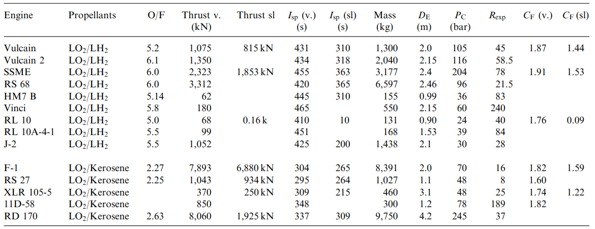
The propulsion database can be found in Section A of the Appendix and a more detailed literature search in their respective reports.

Literature Sources [17]:

Dr. Chudoba’s Project descriptions used to find volume of propellant
Rocket and Spacecraft Propulsion parameter outputs and propellant densities
Design of liquid propellant engines for actual ranges of liquid propellants
Space Propulsion Design and Analysis book

Methods:

Humble Method
Huzel and Huang Method
Building trendlines in Excel from historical engines

Historical Examples for engines:

Table of historical rocket engines, from Vulcain and SSME to the RD-170, with their propellants (liquid oxygen with liquid hydrogen or kerosene), mixture ratio, thrust in vacuum and at sea level, specific impulse, mass, diameter, chamber pressure and other figures. — Figure 14Propulsion Team Historical Engine Database [17]

GStructures

The structures team has compiled several equations regarding thermal loads and useful equations for determining peak temperature as a function of velocity and altitude, based on the aircraft’s geometry and material properties.

A summary of the literature search conducted by the structures team [18]:

Literature Sources (PDF’s and Technical Papers):

Performance study of two-stage-to-orbit Reusable launch vehicle propulsion alternatives.
Comparative Analysis of two-stage-to-orbit Rocket & Airbreathing Reusable Launch Vehicles for Military Applications
Launch Vehicle Design Process: Characterization, Technical Integration, and Lessons Learned.
Development of a Mass Estimating Relationship Database for Launch Vehicle Conceptual Design
Development of a Conceptual Design Weight Estimation Library

Literature Sources (Textbooks):

Space Vehicle Design: Second Edition
Elements of Spacecraft Design
Design Methods for Space Transportation
Future Spacecraft Propulsion Systems: Enabling Technologies for Space Exploration

Equations:

Elements of Spacecraft Design- Chapter #7: Set of equations for basics of preliminary Aerothermodynamic analysis
Development of a Mass Estimating Relationship Database for Launch Vehicle Conceptual Design: Set of empirical equations for weight estimations of a spacecraft

Historical Examples:

Weight parametrization of the Hermes Space vehicle
- Statistical and parametrical methods for weight estimation with an example of Hermes.
Elements of Spacecraft Design:
- Method for Parametric analysis for Aerothermodynamics with a few example problems.

HStability and Control

A summary of the literature search conducted by the stability and control discipline team [19]:

Literature Sources:

Aircraft Flight Dynamics, a lecture series by Stengel provides S&C equations for supersonic and subsonic regimes
Equations and Charts for the Evaluation of the Hypersonic Aerodynamic Characteristics of Lifting Configurations by the Newtonian Theory by Clark and Trimmer provides S&C equations for hypersonic regimes
Flight Determined Stability and Control Characteristics of the M2-F3 Lifting Body and A Correlation Between Flight-Determined Derivatives and Wind-Tunnel Data for the X-24B Research Aircraft are both NASA technical reports by Sim. These both contain stability and control documentation for the two major types of lifting bodies, the flat body X-24B and the round bodied M2-F3. These are used for verification of the methods.
Investigation of the Low-Subsonic Stability and Control Characteristics of a 1/3-Scale Free-Flying Model of a Lifting-Body Reentry Configuration by Hassell is a NASA technical document that contains S&C data for the subsonic range of capsule reentry vehicles. This will be used to investigate if S&C has any major benefits using a lifting body over a capsule.
Airplane Flight Dynamics and Automatic Flight Controls, Vol 1 & 2 by Roskam includes estimations for control derivatives which should be viable even in the hypersonic regime.

Methods and equations:

S&C MATLAB Code evaluating the equations for a set geometry and inputs, performing an analysis of the stability and controllability of the craft for all flight conditions.
$C_{n_{δ_{r}}} = - \frac{(γ_{e 1} + γ_{e 2}) (F_{T} + Δ D)}{δ_{r} q S b}$

Historical examples:

“More than once, vehicle disturbances occurred that were followed by an oscillation sustained by damper augmentation... [which] could produce an unstable closed loop vehicle” (Sim’s analysis of the M2-F3 round lifting body)

IGeometry and Layout

A good resource for developing new geometry from sizing parameters, the following geometric definition section lends itself useful during trade studies for different vehicle geometries [2]. For now, the team intends to use the trapezoidal shape.

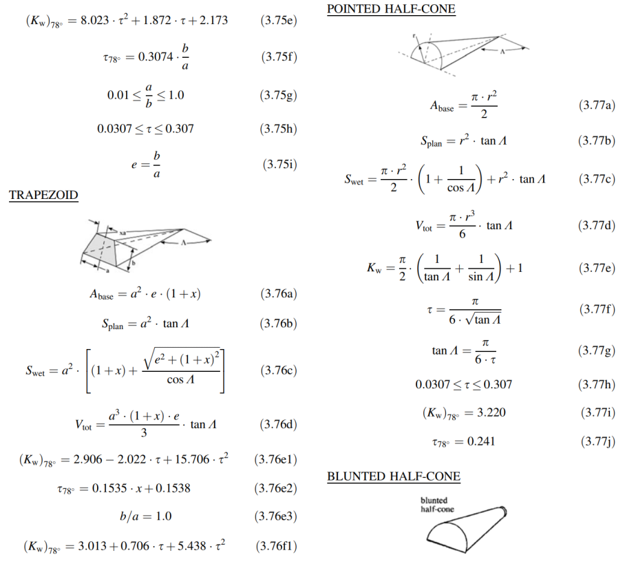
Page of equations for the geometric properties of hypersonic shapes, numbered 3.75 to 3.77, with small drawings of a pointed half-cone, a trapezoid and a blunted half-cone. — Figure 15Geometric Properties of Hypersonic Shapes *[2]*

Below is a summary of the literature research that the CAD discipline has conducted [20]:

Useful references:

Bornemann, W. (1980). Aerodynamic Design Data Book: Orbiter Vehicle STS-1. Rockwell International.
C.F. Ehrlich, F. G. (1986). Preliminary Design and Experimental Invesitgation of the FDL-5S Unmannedd High L/D Spacecraft. Wright-Patterson Air Force Base.
E. Conbeer, D. C. (n.d.). Space Express: Hypersonic Aircraft Design Concept. Princeton: Princeton University.
G.M. Gregorek, D. D. (n.d.). The Design of Four Hypersonic Reconsaissance Aircraft. The Ohio State University.
Lowther, S. (n.d.). Model 176 Art (1). Aerospace Projects Review.
Lowther, S. (n.d.). Model 176 Art (2).

Methods:

OpenVSP
SolidWorks

Historical Examples:

FDL-5
Space Shuttle STS-1

Spotted an error, or want to reply? Email me: leonardo.pinero42 [at] gmail [dot] com